

Join Hack Club Horizons! Ship your projects and fly to your first hackathon →
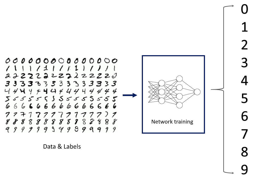
Have you seen all the hype around machine learning and wondered what it's about and how to get started? Well, you're in the right place. In this workshop, we will be training a simple machine learning model to classify handwritten digits.
Getting Started
Prerequisites
An understanding of Python or any other programming language will help greatly with following this tutorial, but you can still do this workshop and learn along the way even if you don't know Python!
Creating the project
We're going to be coding in Google Colab, an online tool that's great for training machine learning models. Make a new Colab project by clicking here.
Coding in Colab
Importing Tensorflow and Dependencies
Let's start off by importing all the required dependencies. We will be using TensorFlow, an open-source machine learning platform. Within TensorFlow we will use the Keras Sequential API, which provides a layer of abstraction on top of all the underlying math theory (though if you are mathematically-inclined, I'd totally recommend diving into the math. Andrew Ng's Coursera course is a great starting place). Using Keras will greatly simplify the process, allowing us to create and train our model with ease.
Add this in your newly-created Colab notebook:
#for rendering pictures and labels properly
%matplotlib inline

import numpy as np
import matplotlib.pyplot as plt

try:
  # %tensorflow_version only exists in Colab.
  %tensorflow_version 2.x
except Exception:
  pass
import tensorflow as tf
Load Training Data
For any machine learning (and particularly deep learning) project, we need data. In our case, we need access to a dataset of thousands of handwritten digits. Lucky for us, MNIST Images does just that. The MNIST dataset was taken from the writing of US Census Bureau officials and high school students, and is commonly used to test/train simple machine learning models. Let's go ahead and load in the dataset using Keras.
nb_classes = 10 #the number of total classes, or categories that there are (0 - 9)

# the data, shuffled and split between tran and test sets
(X_train, Y_train), (X_test, Y_test) = tf.keras.datasets.mnist.load_data()
print("X_train original shape", X_train.shape)
print("y_train original shape", Y_train.shape)
Run the code by clicking the Play button at the left. You should see this print out at the bottom.
Downloading data from https://storage.googleapis.com/tensorflow/tf-keras-datasets/mnist.npz
11493376/11490434 [==============================] - 0s 0us/step
X_train original shape (60000, 28, 28)
y_train original shape (60000,)
Code in Colab is separatered into "cells", so you can separate the code you write and work with different data at different stages. Let's create a new code cell by hovering your mouse on the bottom of the current code cell:

Before preparing the dataset, let us look at some samples of training data. When approaching machine learning problems, visualizing data, when possible, is a great thing to do since it gives useful insights. We can do this using Matplotlib, a Python library that allows us to create simple plots and images from mathematical data.
Note: for the rest of this workshop, when you see one or two code blocks directly followed by an output, assume each code block should be put in a new cell and that you should run the cell to see that output.
In the new cell you created, add:
for i in range(9):
    plt.subplot(3,3,i+1)
    plt.imshow(X_train[i], cmap='gray', interpolation='none')
    plt.title("Class {}".format(Y_train[i]))
#to make sure the spacing between the plots is proper
plt.tight_layout()
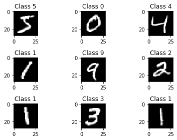
The plt.imshow function converts the digit matrix (all the images are stored as matrices, as we'll soon see) into a visible image. Curious to see what the raw data looks like? Let's take a look. Add these two print statements in a new cell and click the Play button to run the cell.
print(X_train[0])
print("Shape: " + str(X_train[0].shape))
[[  0   0   0   0   0   0   0   0   0   0   0   0   0   0   0   0   0   0
    0   0   0   0   0   0   0   0   0   0]
 [  0   0   0   0   0   0   0   0   0   0   0   0   0   0   0   0   0   0
    0   0   0   0   0   0   0   0   0   0]
 [  0   0   0   0   0   0   0   0   0   0   0   0   0   0   0   0   0   0
    0   0   0   0   0   0   0   0   0   0]
 [  0   0   0   0   0   0   0   0   0   0   0   0   0   0   0   0   0   0
    0   0   0   0   0   0   0   0   0   0]
 [  0   0   0   0   0   0   0   0   0   0   0   0   0   0   0   0   0   0
    0   0   0   0   0   0   0   0   0   0]
 [  0   0   0   0   0   0   0   0   0   0   0   0   3  18  18  18 126 136
  175  26 166 255 247 127   0   0   0   0]
 [  0   0   0   0   0   0   0   0  30  36  94 154 170 253 253 253 253 253
  225 172 253 242 195  64   0   0   0   0]
 [  0   0   0   0   0   0   0  49 238 253 253 253 253 253 253 253 253 251
   93  82  82  56  39   0   0   0   0   0]
 [  0   0   0   0   0   0   0  18 219 253 253 253 253 253 198 182 247 241
    0   0   0   0   0   0   0   0   0   0]
 [  0   0   0   0   0   0   0   0  80 156 107 253 253 205  11   0  43 154
    0   0   0   0   0   0   0   0   0   0]
 [  0   0   0   0   0   0   0   0   0  14   1 154 253  90   0   0   0   0
    0   0   0   0   0   0   0   0   0   0]
 [  0   0   0   0   0   0   0   0   0   0   0 139 253 190   2   0   0   0
    0   0   0   0   0   0   0   0   0   0]
 [  0   0   0   0   0   0   0   0   0   0   0  11 190 253  70   0   0   0
    0   0   0   0   0   0   0   0   0   0]
 [  0   0   0   0   0   0   0   0   0   0   0   0  35 241 225 160 108   1
    0   0   0   0   0   0   0   0   0   0]
 [  0   0   0   0   0   0   0   0   0   0   0   0   0  81 240 253 253 119
   25   0   0   0   0   0   0   0   0   0]
 [  0   0   0   0   0   0   0   0   0   0   0   0   0   0  45 186 253 253
  150  27   0   0   0   0   0   0   0   0]
 [  0   0   0   0   0   0   0   0   0   0   0   0   0   0   0  16  93 252
  253 187   0   0   0   0   0   0   0   0]
 [  0   0   0   0   0   0   0   0   0   0   0   0   0   0   0   0   0 249
  253 249  64   0   0   0   0   0   0   0]
 [  0   0   0   0   0   0   0   0   0   0   0   0   0   0  46 130 183 253
  253 207   2   0   0   0   0   0   0   0]
 [  0   0   0   0   0   0   0   0   0   0   0   0  39 148 229 253 253 253
  250 182   0   0   0   0   0   0   0   0]
 [  0   0   0   0   0   0   0   0   0   0  24 114 221 253 253 253 253 201
   78   0   0   0   0   0   0   0   0   0]
 [  0   0   0   0   0   0   0   0  23  66 213 253 253 253 253 198  81   2
    0   0   0   0   0   0   0   0   0   0]
 [  0   0   0   0   0   0  18 171 219 253 253 253 253 195  80   9   0   0
    0   0   0   0   0   0   0   0   0   0]
 [  0   0   0   0  55 172 226 253 253 253 253 244 133  11   0   0   0   0
    0   0   0   0   0   0   0   0   0   0]
 [  0   0   0   0 136 253 253 253 212 135 132  16   0   0   0   0   0   0
    0   0   0   0   0   0   0   0   0   0]
 [  0   0   0   0   0   0   0   0   0   0   0   0   0   0   0   0   0   0
    0   0   0   0   0   0   0   0   0   0]
 [  0   0   0   0   0   0   0   0   0   0   0   0   0   0   0   0   0   0
    0   0   0   0   0   0   0   0   0   0]
 [  0   0   0   0   0   0   0   0   0   0   0   0   0   0   0   0   0   0
    0   0   0   0   0   0   0   0   0   0]]
Shape: (28, 28)
As you can see, each image is a matrix of size 28 pixels by 28 pixels. Each pixel is a value from 0 (black) to 255 (white), and numbers in between represent various shades of grey.
Preparing the Data for Training
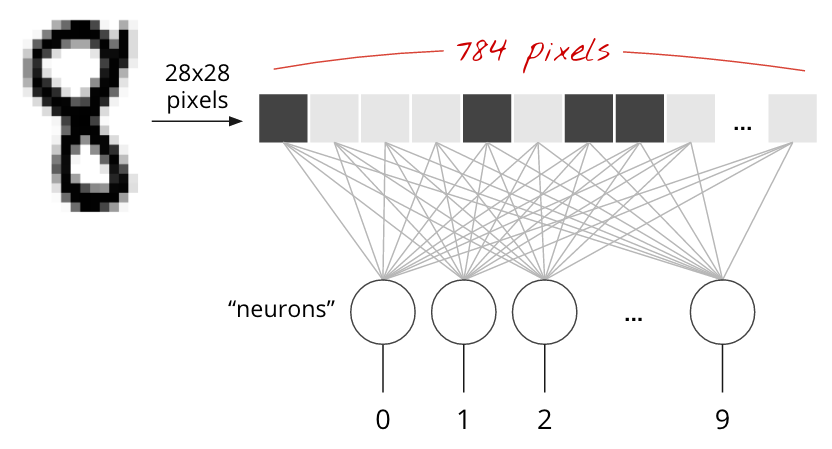
The neural network will take a single vector for training, so the 28x28 images have to be changed into a single 784 dimensional vector. Also we must normalize the pixel values to be from [0->1] instead of [0->255].
Create a new cell, then add the following code:
#the numpy reshape function can be used to reshape an array, as long the new and old
#shapes contain the same amount of elements
X_train = X_train.reshape(60000, 784)
X_test = X_test.reshape(10000, 784)
In order to scale all the [0->255] values to be in the range [0->1], we can simple divide the array itself by 255. With Numpy, simple division is applied element-wise, meaning that every element in the array will be divided by 255. In order for us to be able to do this, however, first we need to make sure that all the numbers are in the correct format: float32.
X_train = X_train.astype('float32')
X_test = X_test.astype('float32')
X_train /= 255
X_test /= 255
Let's check to see that our input matrices now have the correct shape!
print("Training matrix shape", X_train.shape)
print("Testing matrix shape", X_test.shape)
Training matrix shape (60000, 784)
Testing matrix shape (10000, 784)
Notice how the training shape went from (60000, 28, 28) to (60000, 784) - now our X data (input data) is ready to be used! Let's now modify our Y data as well.
Right now, as we saw earlier that the output is simply what number an image is. While this is easy for us to understand, in order for the machine to understand all these categories (0, 1, 2, 3 ... 9), the output needs to be in an array format. For this we can use one hot encoding. Essentially, each unique value (like 1, 2, 3, etc.) is given a "slot" in an array that is the size of the total number of unique values(in this case, there are 10 unique numbers). This allows us to convert a simple label format into a machine-readable array.
0 -> [1, 0, 0, 0, 0, 0, 0, 0, 0, 0]
1 -> [0, 1, 0, 0, 0, 0, 0, 0, 0, 0]
2 -> [0, 0, 1, 0, 0, 0, 0, 0, 0, 0]
3 -> [0, 0, 0, 1, 0, 0, 0, 0, 0, 0]
4 -> [0, 0, 0, 0, 1, 0, 0, 0, 0, 0]
5 -> [0, 0, 0, 0, 0, 1, 0, 0, 0, 0]
6 -> [0, 0, 0, 0, 0, 0, 1, 0, 0, 0]
7 -> [0, 0, 0, 0, 0, 0, 0, 1, 0, 0]
8 -> [0, 0, 0, 0, 0, 0, 0, 0, 1, 0]
9 -> [0, 0, 0, 0, 0, 0, 0, 0, 0, 1]
This is especially useful when your data labels are not numbers. For example, if instead of handwritten digits, we were classifying whether a shirt is green, blue, or red, we could assign each of those colors a slot in an array of size 3.
Red   -> [1, 0, 0]
Blue  -> [0, 1, 0]
Green -> [0, 0, 1]
This isn't too hard to implement from scratch. You can loop through all the data and append any unique elements to a list uniqueElements. Then for each element in the data, you can create a new array the same size as uniqueElements filled with zeros, and then set the spot corresponding to its index in the uniqueElements array to 1. If that sounded confusing, don't worry, since Keras has a function that can do this for us!
Y_train = tf.keras.utils.to_categorical(Y_train, nb_classes)
Y_test = tf.keras.utils.to_categorical(Y_test, nb_classes)
print(X_train[0])
print(Y_train[0])
[0.         0.         0.         0.         0.         0.
 0.         0.         0.         0.         0.         0.
 0.         0.         0.         0.         0.         0.
 0.         0.         0.         0.         0.         0.
 0.         0.         0.         0.         0.         0.
 0.         0.         0.         0.         0.         0.
 0.         0.         0.         0.         0.         0.
 0.         0.         0.         0.         0.         0.
 0.         0.         0.         0.         0.         0.
 0.         0.         0.         0.         0.         0.
 0.         0.         0.         0.         0.         0.
 0.         0.         0.         0.         0.         0.
 0.         0.         0.         0.         0.         0.
 0.         0.         0.         0.         0.         0.
 0.         0.         0.         0.         0.         0.
 0.         0.         0.         0.         0.         0.
 0.         0.         0.         0.         0.         0.
 0.         0.         0.         0.         0.         0.
 0.         0.         0.         0.         0.         0.
 0.         0.         0.         0.         0.         0.
 0.         0.         0.         0.         0.         0.
 0.         0.         0.         0.         0.         0.
 0.         0.         0.         0.         0.         0.
 0.         0.         0.         0.         0.         0.
 0.         0.         0.         0.         0.         0.
 0.         0.         0.01176471 0.07058824 0.07058824 0.07058824
 0.49411765 0.53333336 0.6862745  0.10196079 0.6509804  1.
 0.96862745 0.49803922 0.         0.         0.         0.
 0.         0.         0.         0.         0.         0.
 0.         0.         0.11764706 0.14117648 0.36862746 0.6039216
 0.6666667  0.99215686 0.99215686 0.99215686 0.99215686 0.99215686
 0.88235295 0.6745098  0.99215686 0.9490196  0.7647059  0.2509804
 0.         0.         0.         0.         0.         0.
 0.         0.         0.         0.         0.         0.19215687
 0.93333334 0.99215686 0.99215686 0.99215686 0.99215686 0.99215686
 0.99215686 0.99215686 0.99215686 0.9843137  0.3647059  0.32156864
 0.32156864 0.21960784 0.15294118 0.         0.         0.
 0.         0.         0.         0.         0.         0.
 0.         0.         0.         0.07058824 0.85882354 0.99215686
 0.99215686 0.99215686 0.99215686 0.99215686 0.7764706  0.7137255
 0.96862745 0.94509804 0.         0.         0.         0.
 0.         0.         0.         0.         0.         0.
 0.         0.         0.         0.         0.         0.
 0.         0.         0.3137255  0.6117647  0.41960785 0.99215686
 0.99215686 0.8039216  0.04313726 0.         0.16862746 0.6039216
 0.         0.         0.         0.         0.         0.
 0.         0.         0.         0.         0.         0.
 0.         0.         0.         0.         0.         0.
 0.         0.05490196 0.00392157 0.6039216  0.99215686 0.3529412
 0.         0.         0.         0.         0.         0.
 0.         0.         0.         0.         0.         0.
 0.         0.         0.         0.         0.         0.
 0.         0.         0.         0.         0.         0.
 0.         0.54509807 0.99215686 0.74509805 0.00784314 0.
 0.         0.         0.         0.         0.         0.
 0.         0.         0.         0.         0.         0.
 0.         0.         0.         0.         0.         0.
 0.         0.         0.         0.         0.         0.04313726
 0.74509805 0.99215686 0.27450982 0.         0.         0.
 0.         0.         0.         0.         0.         0.
 0.         0.         0.         0.         0.         0.
 0.         0.         0.         0.         0.         0.
 0.         0.         0.         0.         0.13725491 0.94509804
 0.88235295 0.627451   0.42352942 0.00392157 0.         0.
 0.         0.         0.         0.         0.         0.
 0.         0.         0.         0.         0.         0.
 0.         0.         0.         0.         0.         0.
 0.         0.         0.         0.31764707 0.9411765  0.99215686
 0.99215686 0.46666667 0.09803922 0.         0.         0.
 0.         0.         0.         0.         0.         0.
 0.         0.         0.         0.         0.         0.
 0.         0.         0.         0.         0.         0.
 0.         0.         0.1764706  0.7294118  0.99215686 0.99215686
 0.5882353  0.10588235 0.         0.         0.         0.
 0.         0.         0.         0.         0.         0.
 0.         0.         0.         0.         0.         0.
 0.         0.         0.         0.         0.         0.
 0.         0.0627451  0.3647059  0.9882353  0.99215686 0.73333335
 0.         0.         0.         0.         0.         0.
 0.         0.         0.         0.         0.         0.
 0.         0.         0.         0.         0.         0.
 0.         0.         0.         0.         0.         0.
 0.         0.9764706  0.99215686 0.9764706  0.2509804  0.
 0.         0.         0.         0.         0.         0.
 0.         0.         0.         0.         0.         0.
 0.         0.         0.         0.         0.         0.
 0.         0.         0.18039216 0.50980395 0.7176471  0.99215686
 0.99215686 0.8117647  0.00784314 0.         0.         0.
 0.         0.         0.         0.         0.         0.
 0.         0.         0.         0.         0.         0.
 0.         0.         0.         0.         0.15294118 0.5803922
 0.8980392  0.99215686 0.99215686 0.99215686 0.98039216 0.7137255
 0.         0.         0.         0.         0.         0.
 0.         0.         0.         0.         0.         0.
 0.         0.         0.         0.         0.         0.
 0.09411765 0.44705883 0.8666667  0.99215686 0.99215686 0.99215686
 0.99215686 0.7882353  0.30588236 0.         0.         0.
 0.         0.         0.         0.         0.         0.
 0.         0.         0.         0.         0.         0.
 0.         0.         0.09019608 0.25882354 0.8352941  0.99215686
 0.99215686 0.99215686 0.99215686 0.7764706  0.31764707 0.00784314
 0.         0.         0.         0.         0.         0.
 0.         0.         0.         0.         0.         0.
 0.         0.         0.         0.         0.07058824 0.67058825
 0.85882354 0.99215686 0.99215686 0.99215686 0.99215686 0.7647059
 0.3137255  0.03529412 0.         0.         0.         0.
 0.         0.         0.         0.         0.         0.
 0.         0.         0.         0.         0.         0.
 0.21568628 0.6745098  0.8862745  0.99215686 0.99215686 0.99215686
 0.99215686 0.95686275 0.52156866 0.04313726 0.         0.
 0.         0.         0.         0.         0.         0.
 0.         0.         0.         0.         0.         0.
 0.         0.         0.         0.         0.53333336 0.99215686
 0.99215686 0.99215686 0.83137256 0.5294118  0.5176471  0.0627451
 0.         0.         0.         0.         0.         0.
 0.         0.         0.         0.         0.         0.
 0.         0.         0.         0.         0.         0.
 0.         0.         0.         0.         0.         0.
 0.         0.         0.         0.         0.         0.
 0.         0.         0.         0.         0.         0.
 0.         0.         0.         0.         0.         0.
 0.         0.         0.         0.         0.         0.
 0.         0.         0.         0.         0.         0.
 0.         0.         0.         0.         0.         0.
 0.         0.         0.         0.         0.         0.
 0.         0.         0.         0.         0.         0.
 0.         0.         0.         0.         0.         0.
 0.         0.         0.         0.         0.         0.
 0.         0.         0.         0.         0.         0.
 0.         0.         0.         0.         0.         0.
 0.         0.         0.         0.        ]
[0. 0. 0. 0. 0. 1. 0. 0. 0. 0.]
Building the Neural Network
Now we will build our neural network. The high-level tf.keras API makes this part much easier and does the heavy lifting for us. We will use a simple 3 layer fully-connected network.

In a new cell, add:
model = tf.keras.Sequential([
                              tf.keras.layers.Dense(512, input_shape=(784,)),
                              tf.keras.layers.Activation('relu'),
                              tf.keras.layers.Dropout(0.2),
                              tf.keras.layers.Dense(10),
                              tf.keras.layers.Activation('softmax')
])
model.summary()
Model: "sequential"
_________________________________________________________________
Layer (type)                 Output Shape              Param #
=================================================================
dense (Dense)                (None, 512)               401920
_________________________________________________________________
activation (Activation)      (None, 512)               0
_________________________________________________________________
dropout (Dropout)            (None, 512)               0
_________________________________________________________________
dense_1 (Dense)              (None, 10)                5130
_________________________________________________________________
activation_1 (Activation)    (None, 10)                0
=================================================================
Total params: 407,050
Trainable params: 407,050
Non-trainable params: 0
_________________________________________________________________
Compile the model
When compiing a model, Keras asks you to specify your loss function and your optimizer. The loss function we'll use here is called categorical crossentropy, and is a loss function well-suited to comparing two probability distributions.
Here our predictions are probability distributions across the ten different digits (e.g. "we're 80% confident this image is a 3, 10% sure it's an 8, 5% it's a 2, etc."), and the target is a probability distribution with 100% for the correct category, and 0 for everything else. The cross-entropy is a measure of how different your predicted distribution is from the target distribution. If you are interested in learning more about the math behind cross entropy, feel free to check out this Wikipedia link.
The optimizer helps determine how quickly the model learns, how resistent it is to getting "stuck" or "blowing up". We won't discuss this in too much detail, but "adam" is often a good choice.
model.compile(loss='categorical_crossentropy', optimizer='adam', metrics=['accuracy'])
Training the Model!
It is time to feed the prepared data into our newly created model. This is where the magic happens!
model.fit(X_train, Y_train,
          batch_size=128, epochs=4, verbose=1,
          validation_data=(X_test, Y_test))
Epoch 1/4
469/469 [==============================] - 4s 9ms/step - loss: 0.2838 - accuracy: 0.9189 - val_loss: 0.1467 - val_accuracy: 0.9574
Epoch 2/4
469/469 [==============================] - 4s 8ms/step - loss: 0.1214 - accuracy: 0.9649 - val_loss: 0.0964 - val_accuracy: 0.9710
Epoch 3/4
469/469 [==============================] - 4s 9ms/step - loss: 0.0843 - accuracy: 0.9746 - val_loss: 0.0776 - val_accuracy: 0.9753
Epoch 4/4
469/469 [==============================] - 4s 9ms/step - loss: 0.0638 - accuracy: 0.9807 - val_loss: 0.0700 - val_accuracy: 0.9790


<tensorflow.python.keras.callbacks.History at 0x7f3ab2457da0>
Trying out the Model
We've done it! Our model is now trained and should be able to classify images of digits. Let's check out how accurate our model is! We can do this using the model.evaluate() function.
score = model.evaluate(X_test, Y_test, verbose=0)
print(score)
print('Test score:', score[0])
print('Test accuracy:', score[1])
[0.07004144787788391, 0.9789999723434448]
Test score: 0.07004144787788391
Test accuracy: 0.9789999723434448
Evaluating the Output
It's time for us to make some predictions!
predictions = model.predict(X_test)
print(predictions[0])
[9.8877479e-07 6.1186952e-08 5.3181724e-05 2.1840114e-04 4.6685926e-09
 6.9973555e-07 5.5731461e-11 9.9970931e-01 1.3804106e-06 1.5906311e-05]
Each slot in the one-hot encoded array represents the probability from 0 to 1 that a given image belongs to the slot's class. As you can see in the predictions above, the 7th element has the highest value, meaning that the image most likely is a 7.
predicted_classes = np.argmax(predictions, axis=-1)
print(predicted_classes)
[7 2 1 ... 4 5 6]
# Check which items we got right / wrong
Y_test = np.argmax(Y_test, axis=-1)
correct_indices = np.nonzero(predicted_classes == Y_test)[0]
incorrect_indices = np.nonzero(predicted_classes != Y_test)[0]
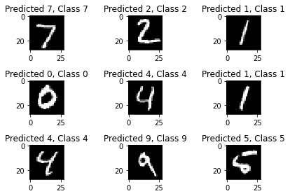
plt.figure()
for i, correct in enumerate(correct_indices[:9]):
    plt.subplot(3,3,i+1)
    plt.imshow(X_test[correct].reshape(28,28), cmap='gray', interpolation='none')
    plt.title("Predicted {}, Class {}".format(predicted_classes[correct], Y_test[correct]))
plt.tight_layout()
plt.figure()
for i, incorrect in enumerate(incorrect_indices[:9]):
    plt.subplot(3,3,i+1)
    plt.imshow(X_test[incorrect].reshape(28,28), cmap='gray', interpolation='none')
    plt.title("Predicted {}, Class {}".format(predicted_classes[incorrect], Y_test[incorrect]))

plt.tight_layout()
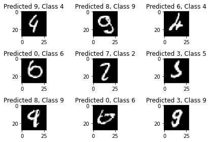
I find it super interesting to see how numbers that even people might mix up causes trouble for our neural network too!
Next Steps!
Congratulations on crafting your first neural network! I hope this project has kickstarted your interest in machine learning. Here are a few ways you can extend this project or use the same process we used in this workshop to solve other problems.
- Connect the model with a website
- Add a digit drawing interface with TensorFlow.js
- Create an MNIST API using TensorFlow Serving
Happy hacking!